In Part 2 we saw that our temperature control process behaved very badly at the low flow rate associated with startup. The root cause of the poor behaviour is that the process behaviour no longer works well with the PID controller. In this section we will look at how to make the process behave better.
In this case, we focus on making the process gain constant across the full range of operating conditions. This is achieved with controller output characterization. This is a lookup table that converts the controller output to a valve position. This can change a linear valve to an equal percent valve, or vise versa. Careful selection of the points in the table will produce a uniform process gain over the entire operating range. This will not address any changes in the process time constant or the dead time.
With a bit of hydraulic modeling and simple process modeling, we can develop a curve that provides a uniform process gain over the entire operating region. It is left as an exercise for the reader to demonstrate how to use the process gain graph to produce a lookup table that yields a constant process gain over the entire range of valve positions. The result, shown below, converts an equal percent valve to an “Increasing Percent” valve.
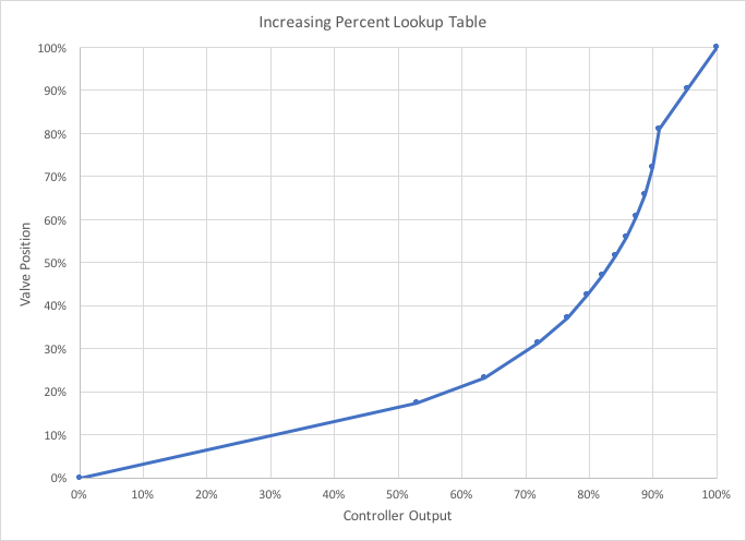
The controller output is needs to be 85% for a 60% valve position. This may be uncomfortable for people accustomed to controller output being in the range of 50 – 80% for normal operation. But this is what is required for uniform process gain over the entire operating region.
The downside to output characterization is that we have no compensation for any changes in the process dead time or time constant. This deficiency will limit the application of output characterization for dead time dominant processes.
The acid test is to see how the new “increasing percent” controller trim behaves at startup conditions. Here, we have the process gain matched nearly perfectly, but there is no compensation for the increased time constant or the dead time.
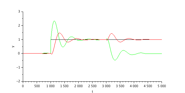
The oscillations are due to the relatively short 40 second response time compared to the 60 second time delay. This performance is probably acceptable at the startup flow rate of 33,000 kg/h, but this cannot be pushed much lower. If the process response was not dominated by a large time delay, the closed loop response would be much less oscillatory.
Next, we will configure the PID controller to accommodate the change in process behaviour.