
Introduction
Equilibrium calculations form the heart of chemical engineering. The most frustrating applications are with ionic solutions where there are a large number of species and many competing reactions.
There is some great software for this, many of which are derived from MINEQL which originated at MIT in the early 1970’s. MINEQL uses a simultaneous solution to the linear material balance equations and the nonlinear equilibrium expressions (refer to Wolery for an explaination of the mathematics).
This short note presents a novel variation of the iterative solution method used in MINEQL. It is hoped that this new algorithm is easier to implement in a spreadsheet or high level programming languages such as SciLab or Python. We will combine concpets in matrix algebra and Taylor series to devise a standard way to approach a difficult problem in chemistry.
Governing equations
The mathematics will be developed using the following set of equilibrium reactions involving the carbonate and sulfide systems. Each reaction has an equilibrium constant K_i and an extent of reaction r_i.
| Reaction | Eqm K and reaction extent r |
| H2S = HS– + H+ | K1, r1 |
| HS– = S-2 + H+ | K2, r2 |
| H2CO3 = HCO3– + H+ | K3, r3 |
| HCO3– = CO3-2 + H+ | K4, r4 |
| H2O = OH– + H+ | K5, r5 |
Precipitation of a solute is not considered.
The reaction stoichimetry is expressed as a matrix S(m,n) where m is the number of reactions and n is the number of species (written as acid dissociation):
| Rxn Name | Equation | H2S | HS– | S-2 | H2CO3 | HCO3– | CO3-2 | OH– | H+ | H2O |
|---|---|---|---|---|---|---|---|---|---|---|
| H2S 1 | H2S = HS– + H+ | -1 | 1 | 0 | 0 | 0 | 0 | 0 | 1 | 0 |
| H2S 2 | HS– = S-2 + H+ | 0 | -1 | 1 | 0 | 0 | 0 | 0 | 1 | 0 |
| Carbonic 1 | H2CO3 = HCO3– + H+ | 0 | 0 | 0 | -1 | 1 | 0 | 0 | 1 | 0 |
| Carbonic 2 | HCO3– = CO3-2 + H+ | 0 | 0 | 0 | 0 | 1 | 1 | 0 | 1 | 0 |
| Water | H2O = OH– + H+ | 0 | 0 | 0 | 0 | 0 | 0 | 1 | 1 | -1 |
The concentration of each species is denoted c_i. The stoichiometry matrix S does not include the solvent species water.
The conservation of mass for each species relates the initial concentration of the species and the extent of each reaction that the species appears in. For example, the concentration of HS- is
[HS-] = [HS-]ic + r1 – r2
A pattern is seen when we take the transpose of the stoichiometry matrix S.
| Species | Initial Conc | r1 | r2 | r3 | r4 | r5 |
|---|---|---|---|---|---|---|
| H2S | [H2S]ic | -1 | 0 | 0 | 0 | 0 |
| HS– | [HS-]ic | 1 | -1 | 0 | 0 | 0 |
| S-2 | [S2-]ic | 0 | 1 | 0 | 0 | 0 |
| H2CO3 | [H2CO3]ic | 0 | 0 | -1 | 0 | 0 |
| HCO3– | [HCO3-]ic | 0 | 0 | 1 | 1 | 0 |
| CO3-2 | [CO32-]ic | 0 | 0 | 0 | 1 | 0 |
| OH– | [OH-]ic | 0 | 0 | 0 | 0 | 1 |
| H+ | [H+]ic | 1 | 1 | 1 | 1 | 1 |
The concentration of each species is related to the initial concentration of each species by the matrix equation

Each of the five equilibrium products are:
- K1 = [HS-] [H+] / [H2S]
- K2 = [S-2] [H+] / [HS-]
- K3 = [HCO3-] [H+] / [H2CO3]
- K4 = [CO3-2] [H+] / [HCO3-]
- K5 = [H+][OH-]
These equations are written in a linear form by taking the logarithm.
- ln K1 = ln [HS-] + ln [H+] – ln [H2S]
- ln K2 = ln [S-2] + ln [H+] – ln [HS-]
- ln K3 = ln [HCO3-] + ln [H+] – ln [H2CO3]
- ln K4 = ln [CO3-2] + ln [H+] – ln [HCO3-]
- ln K5 = ln [H+] + ln [OH-]
We can write the equilibrium expressions using the stoichiometry matrix S:
S (ln c) = ln K
This is where the computational difficulty arrises. The material balances and reaction extents are linear with respect to the species concentration, while the equilibrium expressions are linear with respect to the logarithm of concenentration.
Novel solution method
The MINEQL algorithm uses the logarithm of concentrations as the solution variables (described by Wolery), which makes the equilibrium expression linear. The reaction extent and material balances are expressed as non-linear functions of (ln ci). The material balance expressions are written as exponential functions of (ln ci), and the entries in the Jacobian matrix are complex expression of (ln ci).
We will take a different approach, with the intention of creating a simple recipe for setting up equations for solving equilibrium problems.
Consider the variable x and its logarithm. The two are related by the identity:

We seek a linear approximation (a Taylor series) to relate the variable x and the logarithm of the variable. Note that the derivative is

Since we have estimates of x and ln x at the n iteration level, we can use a Taylor series to write a linear equation for the value of x and ln x at the n+1 iteration level

and since x = exp(ln x), we obtain

The last equation couples the value of the concentration to the logarithm of concentration. This relationship is important because it ensures that concentrations remain positive values. A negative value for a concentration does not impact the solution to the linear system.
This expression is written as:

or in matrix form

where (ln c) is the past estimate for the log of the concentrations.
Given the known values for the right hand side vector b we get a matrix equation of the form
A xn+1 = b
which defines the conservation of mass for each species, equilibrium for each reaction and the Taylor series to relate species concentration and it’s logarithm.
The novel solution method is to write a partitioned matrix equation to describe the iterative solution to the conservation of species mass, equilibrium and the Taylor series for concentration logarithms. The solution vector x comprises the species concentration c, the extent of each reaction r and the logarithm of the species concentration ln c.
![x^{n+1}=\left[ \begin{matrix} c^{n+1} \\ r \\ (\ln{c})^{n+1} \\ \end{matrix} \right]](https://kevindorma.ca/wp-content/ql-cache/quicklatex.com-dcb694fdafebceaaa524c907db8962f5_l3.png "Rendered by QuickLaTeX.com")
and
![A=\left[\begin{matrix} I & S^T & 0 \\ 0 & 0 & S \\ I & 0 & -I \exp{(\ln c)} \\ \end{matrix}\right] \\ b=\left[\begin{matrix} c_{o}\\ \ln{K}\\ \exp{(\ln c)}(1 - (\ln c))\\ \end{matrix}\right]](https://kevindorma.ca/wp-content/ql-cache/quicklatex.com-dfdb28df5a112fce6ef2523c91536e81_l3.png "Rendered by QuickLaTeX.com")
The next guess for each of the unknowns (c, r, (ln c)) is obtained by solving
xn+1 = A-1 b
Example
Refer to the Jupyter notebook below for a working example of this system.
In this example, the initial concentrations of H2S and H2CO3 are 0.00304 and 0.000102 kgmol/m3. The initial guess for all species concentrations is 1 kgmol/m3.
Results
The history of the error (norm[(ln conc)^n+1 – (ln conc) ]) is

Initially, convergence is zero order with respect to log concentration because our initial guesses are extremely poor (concentrations could be off by many orders of magnitude). Each iteration adjusts the concentration by an order of magnitude and adjusts the logarithms by a constant value. Once the concentrations are close to the final value (after 20 iterations), the algorithm displays second order convergence.
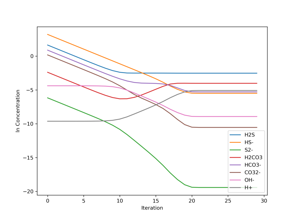
The algorithm requires 25 iterations to produce the converged values.
The converged solution to the equilibrium problem is
| Index | species | concentration | lnConc | neglog10Conc |
|---|---|---|---|---|
| 0 | H2S | 3.036783e-03 | -5.796956 | 2.517586 |
| 1 | HS- | 3.216527e-06 | -12.647208 | 5.492613 |
| 2 | S2- | 5.681526e-17 | -44.709363 | 19.417029 |
| 3 | H2CO3 | 9.681509e-05 | -9.242708 | 4.014057 |
| 4 | HCO3- | 5.184882e-06 | -12.169763 | 5.285261 |
| 5 | CO32- | 2.900148e-11 | -24.263674 | 10.537580 |
| 6 | OH- | 1.190100e-09 | -20.549229 | 8.924417 |
| 7 | H+ | 8.402657e-06 | -11.686963 | 5.075583 |
References
- MINEQL, https://mineql.com/index.html
- T.J. Wolery, CALCULATION OF CHEMICAL EQUILIBRIUM BETWEEN AQUEOUS SOLUTION AND MINERALS: THE EQ3/6 SOFTWARE PACKAGE, UCRL-52658 (1979)
- Acid dissociation constants https://chem.libretexts.org/Ancillary_Materials/Reference/Reference_Tables/Equilibrium_Constants/E1%3A_Acid_Dissociation_Constants_at_25C.